I am constantly on the lookout for fun or interesting datasets to analyze in SVS or VarSeq and recently came across a study looking into inherited cardiac conduction disease in an extended family (Lai et al. 2013). The researchers sequenced the exomes from five family members including three affected siblings and their unaffected mother and an unaffected child of one of the siblings. I’m going to take you through how I was able to analyze, annotate and filter this unique family structure in VarSeq.

The original dataset was downloaded from the European Nucleotide Archive:  ENA Project PRJNA222575. The FASTQ files were aligned using BWA (Burrows-Wheeler Aligner) to generate BAM/BAI files, reads being 76bp paired-end. The five family members’ BAM files were given to GATK Unified Genotyper and variants were called across samples to recognize reference calls between samples that may be important for family variant analysis.

(Note: Here is a link to a blog written by Dr. Bryce Christensen concerning research design set-up and VCF file formats: Have you ever had a bad experience with a VCF file?)

The multi-sample VCF file was imported into an empty VarSeq project. VarSeq does come with Family Trio Analysis templates, but since this is a unique family structure a new workflow is more appropriate.

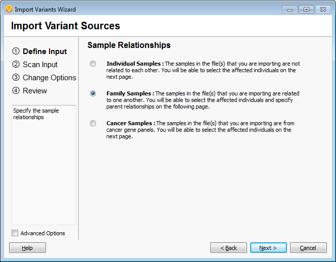
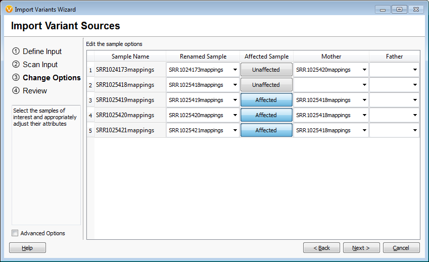
When importing the samples into an empty VarSeq project the first window asks if the samples are related and in this case “family” was selected to indicate they were related. The second window asks which samples are the mother and father and affection status. This family is missing the father and has 2 mothers as the second unaffected individual is a grandson. This information was specified as the pedigree in VarSeq and the data is loaded into the empty project, Figures 1 and 2. The analysis started with 688,928 variants across the five family members.

Figures 1 and 2 Importing Family Samples

(Note: It is also possible to analyze a unique family structure in the “individuals” or unrelated sample format. It is a matter of preference in this case, it will not affect the available functions or filtering. I happen to be a fan of the family labels!)

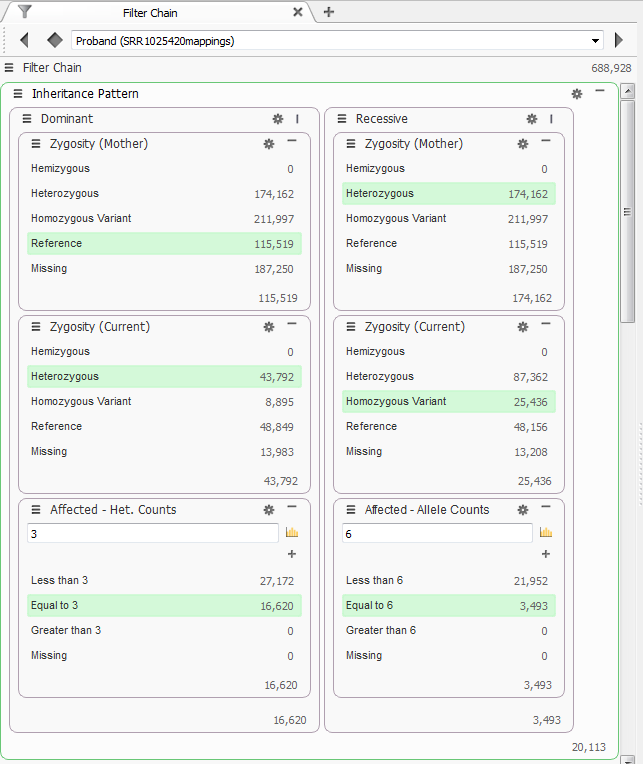
With this pedigree VarSeq indicates the three affected individuals as “Probands” and the unaffected mother as “Mother” and the unaffected grandson as “Child”. The first filter chain I set-up specified different modes of inheritance, Dominant and Recessive. After using the Compute Zygosity State function I used the Mother’s zygosity state to identify variants that were “Reference” and the Probands’ zygosity state as “Heterozygous.” For the recessively inherited variants, Mother was set to “Heterozygous” and the Probands to “Homozygous.” The final filter added to this set was to run the Compute Additional Data function for Allele Counts. This will count the variants across the family and just in affected individuals. The last filter was to specify the number of alleles in affected individuals, for dominant inheritance pattern this is at least 3, one for each affected individual, for the recessive inheritance pattern this is 6 because each affected individual must have 2 alleles to show the phenotype. Through these 2 inheritance patterns 20,113 variants remained from the originally imported 688,928 variants, Figure 3.

The next filter card eliminated non-synonomous variants; this information for each variant is gained from annotating against a gene track. For this family I used the RefSeq 105 Gene Track, annotating against a gene track also gives information about sequence ontology, genes and variant effect. The Variant “Effect” information is used to identify only those variants that are loss of function or missense.

(Note: Gabe Rudy Blog Post about RefSeq Genes: RefSeq Genes: Updated to NCBI Provided Alignments and Why You Care)

Next variants found within segmental duplications were removed from the dataset using the UCSC Genomic Super Dups Track and variants that were found in dbSNP Common track were removed from the dataset. The researchers were looking for a rare variant in the family, so as indicated in the Lai et al. 2013 paper, using the information from 1000 Genomes for the Asian population variants with a minor allele frequency of <0.05 and considered missing were kept.

Figure 3 Dominant and Recessive Inheritance Filters

PhastCons conservation scores were used from the 100way vertebrate information contained in the dbNSFP Functional Predictions track, to remove variants that had a PhastCons score of <0.25. This score looks at how conserved areas of the genome are between a set of taxa. In this case, 100 vertebrate genomes were aligned and conservation scores generated across the 100 species. PhastCons scores range from 0-1 with a value closer to one being highly conserved and closer to zero being less conserved across taxa. PhastCons looks at moderately sized regions; the calculation includes a Hidden Markov Model with data-estimated substitution rates under a neutral model of evolution. Siepel et al. 2005

Variants predicted to be damaging were selected as the next filter, this information was annotated from dbNSFP Functional Predictions and an overall scoring of three or more algorithms that showed the variants as damaging or unknown were selected to pass the filter. This annotation source has precomputed scores for 5 separate functional prediction algorithms including: SIFT, Polyphen, MutationTaster, Mutation Assessor, and FATHMM. This resulted in 31 damaging variants found in the probands.

The final filter in the dataset was applied to further filter variants using the PhoRank calculation found in the new VarSeq release 1.1.1. This is modeled after Phevor Singleton et al. 2014 and the implementation in VarSeq allows researchers to search for a list of phenotypes associated with the disease of interest. It combines information from various bioinformatics tools including Human Phenotype Ontology, Mammalian Phenotype Ontology, Disease Ontology and Gene Ontology. Gene information is needed for each variant as the function queries the databases based on gene information. The final information provided is a PhoRank score for the gene, and variant being cross reference with the given search terms. For this disease, the following search terms were applied: heart block, arrhythmia, and atrial fibrillation. The PhoRank scores higher than 0.75 were kept which concluded with 7 variants found in the dataset, all of these variants coming from the dominant inheritance pattern, Figure 4.

Figure 4 PhoRank Information and Filter

These seven variants included one variant found in the gene LMNA, lamin A/C, which was also indicated in the paper by Lai et al. 2013 as the most likely causal variant in the family. Lamin proteins are believed to be involved in nuclear stability, chromatin structure and gene expression. Lai et al. showed with additional cellular work that the variant (NM_005572, c.G695T, G232V) which produces a glycine-to-valine substitution led to extreme conformational changes in the final protein product. They also continued sequencing individuals with cardiac conduction disease and found this variant in 115 patients with atrial fibrillation. You can see the variant in an affected and unaffected individual using Genome Browse which is fully integrated into VarSeq, Figure 5.

Figure 5 Genome Browse view of likely causal variant in LMNA

VarSeq 1.1.1 is a powerful research tool to identify variants in family trios, unrelated individuals, gene panels and unique family structures as well! Here is a list of all the new features included in the recent release of VarSeq: VarSeq 1.1.1 Release Notes.  I hope you’ve learned a little something more about VarSeq from this blog and if you’re interested in a trail or other Golden Helix product SNP and Variation Suite please contact [email protected].